
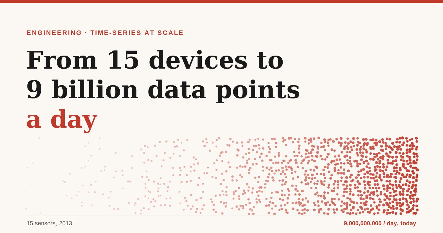
From 15 devices to 9 billion data points a day
Engineering · Time-series at scale

A decade-long detour that began with a parallel port and a row of LED bulbs, and ended with a single self-hosted server quietly absorbing nine billion telemetry messages every day. This is the messy, honest version - every wall we hit, and how we climbed over each one.
By the engineering team · ~15 min read
There is a particular kind of magic in making a piece of software reach out of the screen and move something in the physical world. A relay clicks. A motor spins. A light comes on across the room because of a line of code you wrote. I have been chasing that feeling for more than ten years, and it is the thing that quietly led us to building a system that now handles billions of data points a day without breaking a sweat.
This post is the long version of that journey. Not the polished “we architected a scalable platform” version, but the real one - the part where we made naive choices, hit walls, threw away work, and then went back to the drawing board more times than we would like to admit. If you are building anything in IoT, time-series, or high-ingest telemetry, hopefully our scar tissue saves you some of your own.
2013: the parallel port and a row of LED bulbs
Most motherboards back then still shipped with a parallel port - the wide DB-25 connector that everyone used for dot matrix printers and almost nobody thought about. I was fascinated by how a printer worked: the print head is just an array of tiny pins, and the computer fires those pins in precise patterns by toggling individual data lines on that port. Software, turning into motion, turning into dots on paper.
And the obvious-in-hindsight thought hit me: if I can control the pins on a print head, why can’t I use the exact same signals to control anything else? A pin firing is just a voltage going high. A heater doesn’t care whether the bit that switched it on was meant for a printer.
So I stripped the wires of a parallel cable, put an LED on each data line, and watched them blink as I toggled the port from code. That was the “hello world.” Then I made it do something real: an LED shining onto an LDR (a light-dependent resistor), the LDR switching a small pilot relay, and that pilot relay driving a much bigger contactor rated for real current. With that chain I was switching a room heater and the lights in my house from a program on my PC.
The optocoupling was crude - an LED pointed at a light sensor is about as low-tech as galvanic isolation gets - but conceptually it was exactly right: keep the delicate logic side and the dangerous mains side electrically separate, and let a tiny signal command a big load.
It worked. And then, as these things go, life moved on and the idea went dormant for almost a decade.
2023: denim, dryers, and 15 little ESPs
Fast forward to 2023. By then I had spent years inside factories working on productivity - optimising systems and processes, squeezing out inefficiency on the production side. One of the problems that landed on my desk was in a denim finishing facility: drying denim bottoms, more than 600 pairs at a time.
Temperature in the dryer turned out to be a sneaky, high-stakes variable. Get the exhaust temperature wrong and the garment could shrink - we are talking up to two inches of length lost on a finished pair. At that scale, an uncontrolled temperature swing isn’t a rounding error, it’s a quality incident measured in rejected stock.
So the old itch came back, this time with much better hardware. Instead of a parallel port I now had the ESP - a cheap, WiFi-capable microcontroller. I built a small module to measure the dryer exhaust temperature so we could correlate it with the quality parameters of the denim coming out. We installed 15 of these devices, each sending a temperature reading every second.
The architecture was about as simple as it gets:
The ESP fires an HTTP
POSTto a server, once per reading.A PHP backend receives the call and writes the value to a database.
A visualisation page reads from that database so I could watch the temperatures live.
It ran for two months and it genuinely worked. Encouraged, I expanded the idea: I started measuring sewing machine output as well, and rolled the devices out across 20 assembly lines.
And that is exactly when we hit the first wall.
The bottleneck
Every API call was one database write. On shared hosting, the provider throttled the database the moment our write volume climbed. The APIs started timing out. The whole pretty setup fell over - not because the idea was wrong, but because “one HTTP request, one synchronous DB write” does not survive contact with scale.
Every API call was one database write. On shared hosting, the provider throttled the database the moment our write volume climbed. The APIs started timing out. The whole pretty setup fell over - not because the idea was wrong, but because “one HTTP request, one synchronous DB write” does not survive contact with scale.
It was a side quest at the time, so we let it drop. But the lesson stuck: the database, and how you talk to it, is going to be the thing that decides whether you live or die.
The real beginning: looking at the utility side
Later that year, my attention shifted. For five years I had optimised processes - how things get made - but I had never seriously looked at the utility side: the power, the compressed air, the steam, the water. The boring infrastructure that every factory pays for and almost nobody instruments. When I started staring at the opex, the utility line drew my attention in a way it never had before. There was clearly an enormous amount of waste hiding in plain sight, and almost nobody was watching it second by second.
So we did what we did before: built a prototype, and started investigating properly. What open-source stacks exist? What is the tech actually doing under the hood? One decision we made early and have never regretted: the whole thing had to be built on a completely open-source stack. I had watched systems get held hostage by closed, proprietary models - you build your whole operation on top of someone’s black box, and then you discover you don’t really own any of it. Never again.
The first “real” architecture - and the 6,000-a-minute wall
This time we started with the right transport. We chose MQTT, because it is the de-facto industry standard for this kind of telemetry - lightweight, pub/sub, built for unreliable networks and constrained devices. (Thank god. That one choice has aged beautifully; we are still on it.)
For the rest of the stack:
PostgreSQL for the backend store.
A Python script as the middleman - pulling messages off MQTT and writing them into Postgres.
I was happy. It was clean, it was ours, it was open source. And it was all fun… until we hit roughly 6,000 messages per minute. Then everything started throttling, and when we pulled it apart, the problems were textbook:
No multithreading. The Python middleman processed messages essentially serially. It simply could not keep up.
Postgres was hosted online, so every transaction paid a network round-trip of latency on top of its own work.
Every transaction opened its own connection. This was the genuinely scary one. At 6,000 messages a minute we were making and destroying 6,000 connections a minute. Connection setup and teardown is expensive; we were spending most of our budget on handshakes instead of actual writes.
We did the obvious first fix - persistent connections, so we stopped paying the connection-churn tax. It helped, but not nearly as much as we hoped, because the dominant cost was now the latency between the app and a remotely hosted database. Every write still had to travel.
We took a brief detour to InfluxDB, the obvious “time-series database” answer. But the specific offering we were on came with limitations that didn’t fit, and we switched back to Postgres.
TimescaleDB: the first real gamechanger
Then we learned about TimescaleDB, and it changed everything.
The beautiful part is that TimescaleDB is not a different database - it is a PostgreSQL extension. So we didn’t have to abandon the database we already understood, the SQL we already wrote, or the ecosystem we already relied on. We just taught Postgres how to be brilliant at time-series data. Under the hood it shards your data into time-based chunks (“hypertables”), which keeps the indexes that matter small and hot, and makes both inserts and time-range queries dramatically faster.
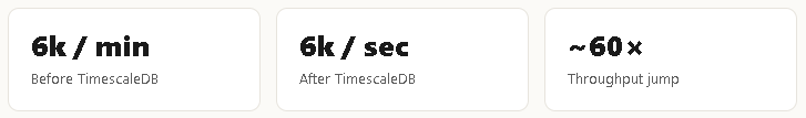
We went from 6,000 messages per minute to 6,000 messages per second. Same conceptual stack, roughly a 60× jump, just by putting the right tool under the writes.
That put us at around 8–9 million messages a day. A real system, finally. But we had quietly written a much bigger number on the whiteboard as our internal benchmark: one billion messages per day. So we went back to the drawing board and started interrogating every single stage of the pipeline.
Re-thinking ingestion: the broker bake-off
If the database was now strong, the next question was the front door: the MQTT broker that has to hold thousands of device connections open and not fall over. We didn’t guess - we evaluated a lot of options, both open-source and cloud-managed:
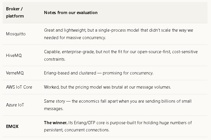
We settled on EMQX. The reason is the same reason VerneMQ was on the list and the same reason telecom systems were historically built on it: Erlang/OTP. The Erlang runtime was designed for systems with millions of lightweight, concurrent processes that need to stay up - exactly the shape of “thousands of devices each holding a persistent connection.” EMQX rides on that core, so concurrency that would topple a single-threaded broker is just a normal Tuesday for it.
The number that still surprises people
Moving ingestion onto self-hosted EMQX instead of a managed cloud IoT platform took our projected ingestion cost from somewhere around USD 300,000 to effectively zero - because at this point we had bought our own server, and the broker is open source. On a managed per-message platform, our volume would have quietly bled us dry.
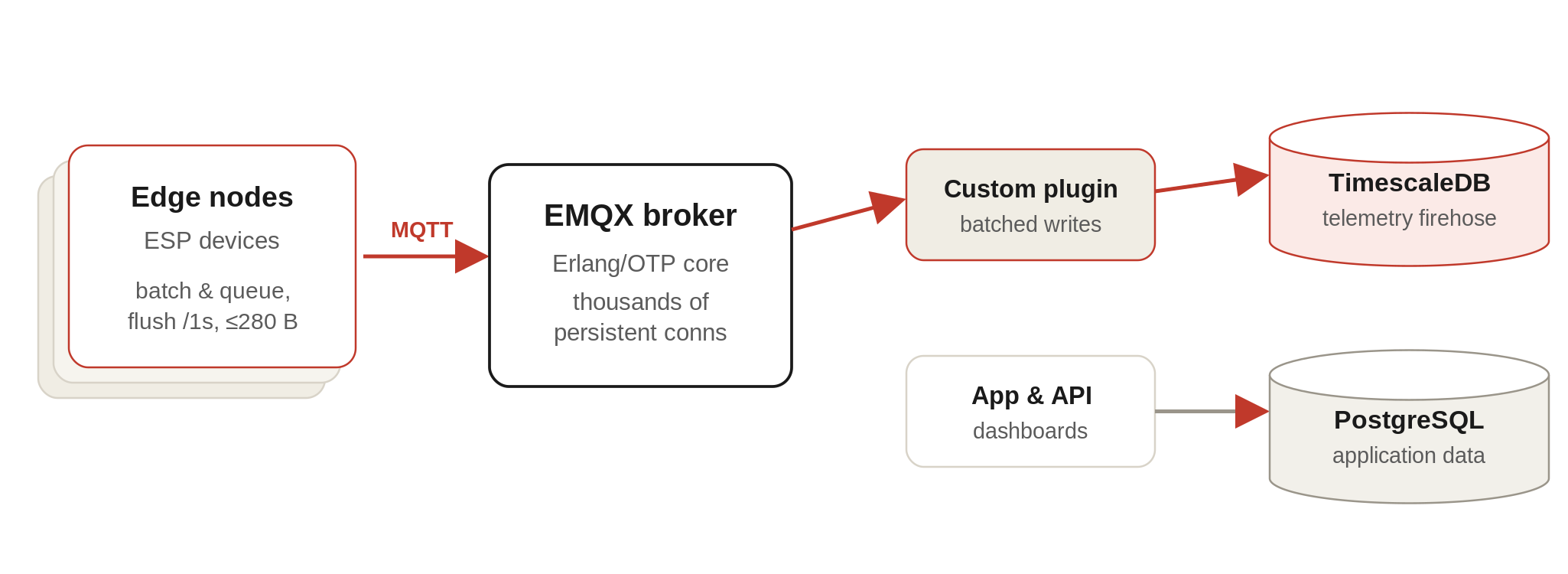
For the last mile from broker to database, we wrote a custom EMQX plugin that takes the incoming messages and writes them into TimescaleDB directly in a manner that is suited for faster retrieval and aggregation - no fragile intermediate hop.
Two databases, on purpose
Somewhere in here we accepted a truth we had been resisting: one database is not going to do both jobs. So we split it:
A TimescaleDB store for the firehose of telemetry data.
A plain PostgreSQL store for normal application data - users, devices, config, the things that are read and written at human speed.
Different access patterns, different tuning, different failure modes. Trying to serve both from one box is how you end up with an application query getting stuck behind a million-row ingest.
Why we bought our own server (and fired the cloud)
This is the decision people argue with most, so let me be specific about why, because it was not ideology - it was IOPS.
Our workload is a relentless storm of small writes. That makes us almost entirely IOPS-bound (input/output operations per second), not CPU-bound or bandwidth-bound. And here is the thing nobody tells you until you’re bleeding:
AWS EC2 with general-purpose EBS was the worst fit imaginable for us. The IOPS flatlined at around 16,000 in the best case - and for our write pattern, 16,000 IOPS is nothing. Our app would eat that for breakfast and ask for more.
We could have gone for higher-tier provisioned IOPS or a fully managed database, but the cost for our specific, high-IOPS use case was simply absurd.
So we bought our own server. On bare metal we got to choose our own storage and tune the machine to the workload instead of paying a premium to be capped. Which led directly to the next rabbit hole.
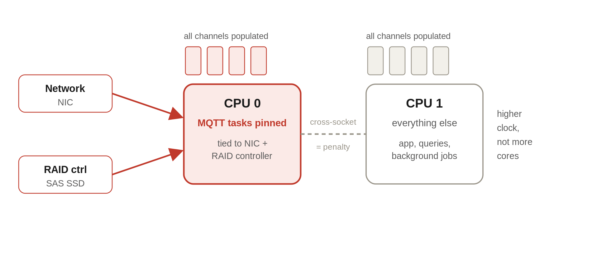
Going down to the metal: packets, sockets and CPU pinning
Once you own the box, you can optimise things the cloud never lets you touch. We went deep into how a packet actually flows through the machine: which CPU socket is wired to the network interface, which one handles the storage controller, where the interrupts land, how data crosses between sockets.
This is NUMA (non-uniform memory access) territory. On a multi-socket server, memory and PCIe devices are “closer” to one socket than the other, and a thread running on the wrong socket pays a penalty crossing the interconnect to reach the NIC or the RAID controller. So we pinned all our MQTT-related work to CPU 0, because CPU 0 was the socket directly tied to the network interface and the RAID controller. Keep the network-to-storage path on the same socket, and you stop paying the cross-socket tax on every single message.
Picking the right CPU, and waking up all the RAM
Two more metal-level choices mattered more than we expected. The first was the CPU itself. At a fixed power package limit you can’t have everything - you trade more cores against higher clock speed, because the same thermal and power envelope has to be shared either way. For a lot of workloads, more cores wins. Ours is not one of them: the hot path is a tight, latency-sensitive loop of receiving a message and committing a write, and that path cares about how fast a single core can churn through it. So we deliberately chose higher per-core clock speed over a higher core count, within the same power budget. Faster cores, fewer of them, and the per-message latency dropped.
The second was embarrassingly simple and embarrassingly effective: memory channels. It is tempting to drop in one big DIMM and call it done, but a modern CPU has multiple memory channels and only reaches its full memory bandwidth when those channels are all populated. We had effectively been driving a multi-lane highway with one lane open. We reconfigured the server to spread RAM across every memory channel instead of stuffing capacity into a single slot - same total memory, but now the CPU could actually pull from it in parallel. For a workload constantly shuttling buffers between the network, memory and disk, that extra bandwidth is free throughput.
That body of work - pinning, the CPU choice, and the memory reconfiguration - took us to 600 million MQTT messages per day. Real progress - but still well short of the billion we’d promised ourselves. So, again, back to the drawing board.
Marginal gains: where the billion actually came from
There’s a story we kept coming back to. When Dave Brailsford took over British Cycling, he didn’t look for one magic 10× improvement. He looked for a hundred tiny 1% improvements - the pillow they slept on, how they washed their hands, the seat fabric - on the theory that all those marginal gains compound. British Cycling went on to dominate the Olympics, and Team Sky won the Tour de France. That was our model for the final stretch. No single hero fix. Just relentless 1% gains.
1. Batch the writes
Instead of writing each message as its own transaction, we moved to batched writes - accumulate many readings and commit them together. Every transaction has fixed overhead; amortise that overhead across hundreds of rows and the per-message cost collapses.
2. The right disks
We moved all our databases onto SAS SSDs with serious IOPS headroom. The gap here is almost comical when you write it down:
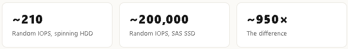
For an IOPS-bound workload, this is not a tweak, it’s a different universe. A spinning disk physically has to move a head and wait for the platter to rotate; an SSD just… doesn’t.
3. Stop sending so many tiny messages
The final, subtle one was at the edge. Originally, every single data point was its own MQTT message - the same “one event, one message” sin from the very first PHP project, just at a higher tier. So we changed the firmware’s behaviour: the edge device now queues readings for a second and sends them in a single batched payload, flushing either every second or when the buffer reaches 50% of the allowed packet size - whichever comes first.
Why 50%? Because the other half is reserved for protocol overhead, and because we have to survive badly configured networks in the real world. We cap our payloads at about 280 bytes. The reasoning:
The minimum IPv4 datagram every host must be able to handle is 576 bytes. In a healthy network you’d never get near that floor, but in a highly misconfigured industrial environment, the effective packet size really can drop to it.
Subtract IP, TCP and MQTT headers, then leave generous room for overhead, and you land at a payload ceiling around 280 bytes that will get through almost anywhere without fragmentation.
The combination - batching at the edge, batching at the write, and keeping every packet small enough to never fragment - meant we were now moving far more data points per message, and every message was reliable.
Where we are today
All those marginal gains compounded exactly like the cycling team’s did. We blew past our own one-billion goal, and kept going.
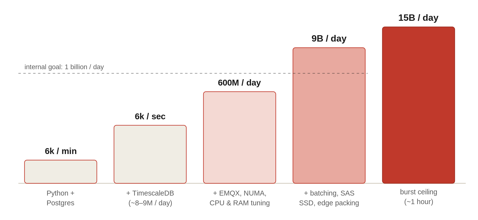
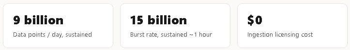
Today we sit comfortably at 9 billion transactions per day, sustained. If we talk about bursts, we can hold a 15-billion-per-day rate for about an hour. And honestly - if we ever genuinely reach that ceiling on a sustained basis, that’s a wonderful problem to have. It means the thing is being used. We’ll go back to the drawing board, like we always do, and scale the next stage.
All of this runs on a self-hosted, fully open-source stack: MQTT over EMQX, a custom ingest plugin, TimescaleDB for telemetry and PostgreSQL for application data, on a NUMA-tuned bare-metal server with SAS SSDs - for effectively zero licensing cost, where the cloud equivalent was quoted in the hundreds of thousands.
What’s next
We are currently tuning the database layer specifically for NVMe - the next jump in storage, where the bottleneck moves off the SAS interface entirely and the queue depths and parallelism look completely different from what we tuned for on SAS SSD. There’s a whole post in that alone, and we’ll be back with a detailed write-up once we’ve learned what it has to teach us.
The lessons, if you skipped to the end
The database and how you talk to it decides everything. Our very first failure and our biggest wins were all about writes: connection churn, latency, batching, the right disk.
“One event, one message, one write” doesn’t scale. Batch at the edge, batch at the broker, batch at the write. We learned this lesson twice before it stuck.
Use the right tool, not a different tool. TimescaleDB let us get 60× without leaving Postgres. Sometimes the upgrade is an extension, not a rewrite.
Know your bottleneck’s units. We were IOPS-bound, not CPU- or bandwidth-bound. Once we named that, every decision - bare metal over EC2, SAS SSD over HDD, NUMA pinning - got obvious.
Cloud is not automatically cheaper or faster. For a specific, brutal, high-IOPS workload, owning the metal took us from a $300k quote to roughly zero, and let us tune things the cloud would never expose.
Marginal gains are real. There was no single 10× fix after TimescaleDB. There were a dozen 1% fixes that compounded into 15×.
Open source is freedom. Every piece of this is something we own and can tune. We have never been one vendor decision away from being held hostage.
It started with LED bulbs glued to a parallel cable, trying to prove that a printer signal could switch a heater. More than a decade later the same stubborn idea - that software should be able to reach out and command the physical world - is moving nine billion data points a day. The fascination never changed. Only the bottlenecks did.